13 Joint quantities and complex data types
\(\DeclarePairedDelimiter{\set}{\{}{\}}\) \(\DeclarePairedDelimiter{\abs}{\lvert}{\rvert}\)
Quantities of more complex types can often be viewed and represented as sets (that is, collections) of quantities of basic and possibly different types.
13.1 Joint quantities
A simple collection of quantities of basic types, for instance “age, sex, nationality”, usually does not have any new mathematical properties appearing just because we’re considering those quantities together. We shall call such a collection a joint quantity. Note that a “joint quantity” it is still a quantity, but not a quantity of a basic type.
The values of a joint quantity are just tuples of values of its basic component quantities. Its domain is the Cartesian product of the domains of the basic quantities.
Consider for instance the age, sex1, and nationality of a particular individual. They can be represented as an interval-continuous quantity \(A\), a binary one \(S\), and a nominal one \(N\). We can join them together to form the joint quantity “(age, sex, nationality)” which can be denoted by \((A,S,N)\). One value of this joint quantity is, for example, \((25\,\mathrm{y}, {\small\verb;F;}, {\small\verb;Norwegian;})\). The domain could be
1 We define sex by the presence of at least one Y chromosome or not. It is different from gender, which involves how a person identifies.
\[ [0,+\infty)\times \set{{\small\verb;F;}, {\small\verb;M;}} \times \set{{\small\verb;Afghan;}, {\small\verb;Albanian;}, \dotsc, {\small\verb;Zimbabwean;}} \]
Discreteness, boundedness, continuity
A joint quantity may not be simply characterized as “discrete”, or “bounded”, or “infinite”, and so on. Usually we must specify these characteristics for each of its basic component quantities instead. Sometimes a joint quantity is called, for instance, “continuous” if all its basic components are continuous; but other conventions are also used.
Consider again the examples of § 12.1.1. Do you find any examples of joint quantities?
13.2 Complex quantities
We shall call “complex quantity” a quantity that is not of a basic type, nor a collection of quantities of basic type, that is, a joint quantity.
Familiar examples of complex quantities are vectorial quantities from physics and engineering, such as location, velocity, force, torque. Other examples are images, sounds, videos.
Note that a complex quantity may be represented as a collection of quantities of basic type. This collection, however, is “more than the sum of its parts”, in the sense that it has new mathematical properties that do not apply or do not make sense for the single components.
Consider for example a 4 × 4 monochrome image, represented as a grid of 16 binary quantities \(0\) or \(1\). Three possible values could be these:

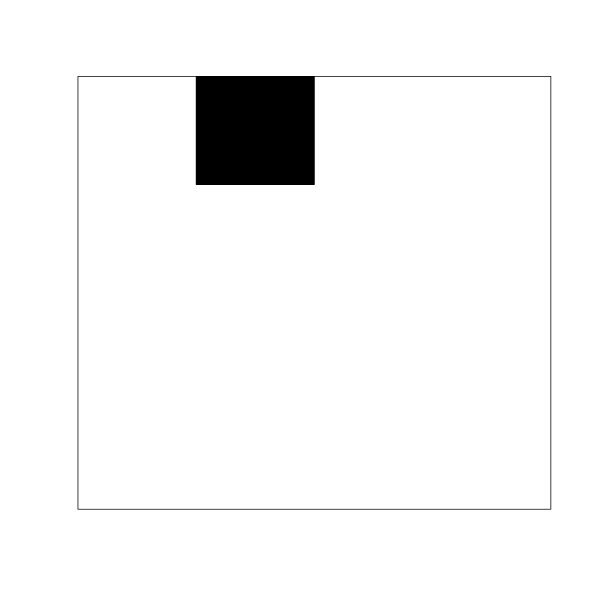
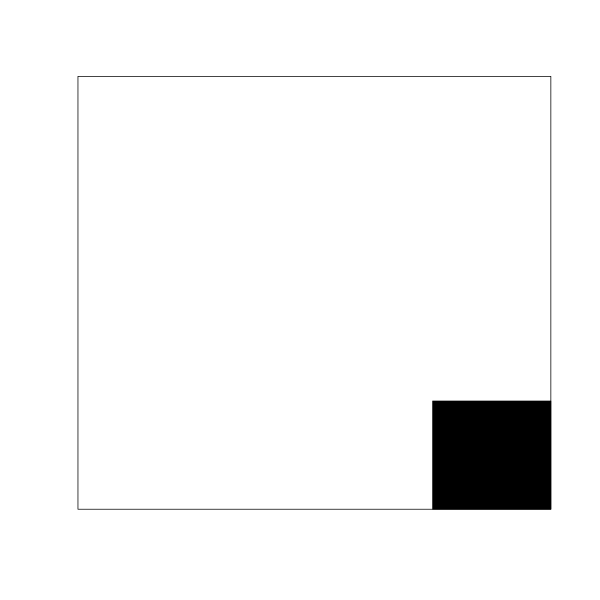
We can numerically represent these images as the matrices
\(\begin{psmallmatrix}1&0&0&0\\0&0&0&0\\0&0&0&0\\0&0&0&0\end{psmallmatrix}\), \(\begin{psmallmatrix}0&1&0&0\\0&0&0&0\\0&0&0&0\\0&0&0&0\end{psmallmatrix}\), \(\begin{psmallmatrix}0&0&0&0\\0&0&0&0\\0&0&0&0\\0&0&0&1\end{psmallmatrix}\).
With this representation, this quantity is made to correspond to 16 binary digits, or in other words 16 binary quantities.
From the point of view of the individual binary quantities, these three values are “equally different” from one another: where one of them has grid value \(1\), the others have \(0\). But properly considered as images, we can say that the first and the second are somewhat more “similar” or “closer” to each other than the first and the third. This similarity can be represented and quantified by a metric over the domain of all such images. This metric involves all basic binary quantities at once; it is a new mathematical property that does not belong to any of the 16 binary quantities individually.
More generally, complex quantities have additional, peculiar properties, represented by mathematical structures, which distinguish them from joint quantities; although there is not a clear separation between the two.
These properties and structures are very important for inference problems, and usually make them computationally very hard. Machine-learning methods are important because they allow us to do approximate inference on these kinds of complex data. The peculiar structures of these data, however, are often also the cause of striking failures of some machine-learning methods, for example the reason why they may classify incorrectly, or why they may classify correctly but for the wrong reason.