20 Populations and variates
\(\DeclarePairedDelimiter{\set}{\{}{\}}\) \(\DeclarePairedDelimiter{\abs}{\lvert}{\rvert}\)
20.1 Collections of similar quantities: motivation
In the latest chapters we gradually narrowed our focus on a particular kind of inferences: inferences that involve collections of similar quantities, each of which can be simple, joint, or complex. “Similar” means that all these quantities have a similar meaning and measurement procedure, and therefore have the same domain. For instance, each quantity might have possible values \(\set{{\small\verb;urgent;}, {\small\verb;non-urgent;}}\); or possible values between \(0\,\mathrm{\textcelsius}\) and \(100\,\mathrm{\textcelsius}\). These quantities can be considered different “instances” of the same quantity, so to speak. We saw an example in the three-patient hospital scenario of § 17.4, with the three “urgency” quantities \(U_1\), \(U_2\), \(U_3\), corresponding to the urgency of three consecutive patients. Here are other examples:
- Stock exchange
- We are interested in the daily change in closing price of a stock, during 1000 days. Each day the change can be positive (or zero), or negative.

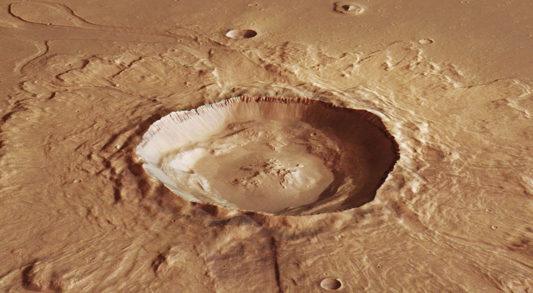
- Mars prospecting
- Some robot examines 1000 similar-sized rocks in a large crater on Mars. Each rock either contains haematite, or it doesn’t contain haematite.
- Glass forensics
- A criminal forensics department has 215 glass fragments collected from many different crime scenes. Each fragment is characterized by a refractive index (between \(1\) and \(\infty\)), a percentage of Calcium (between \(0\%\) and \(100\%\)), a percentage of Silicon (ditto), and a type of origin (for example “from window of building”, “from window of car”, and similar).

It is easy to think of many other and very diverse examples, with even more complex variates, such as images or words. We shall now try to abstract and generalize this similarity.
20.2 Units, variates, statistical populations
Consider a large collection of entities that are somehow similar to one another, as in the preceding examples. We shall call these entities units. Units could be, for instance:
- physical objects such as cars, windmills, planets, or rocks from a particular place;
- creatures such as animals of a particular species, or human beings, maybe with something in common such as geographical region; or plants of a particular kind;
- automatons having a particular application;
- software objects such as images;
- abstract objects such as functions or graphs;
- the rolls of a particular die or the tosses of a particular coin;
- the weather conditions on several different days.
These units are similar to one another in that they have some set of attributes1 common to all. These attributes can present themselves in a specific number of mutually-exclusive guises. For instance, the attributes could be:
1 The term features is frequently used in machine learning
- “colour”, each unit being, say,
green,blue, oryellow; - “mass”, each unit having a mass between \(0.1\,\mathrm{kg}\) and \(10\,\mathrm{kg}\);
- “health condition”, each unit (an animal or human in this case) being
healthyorill; or maybe being affected by one of a specific set of diseases; - containing something, for instance a particular chemical substance;
- “having a label”, each unit having one of the labels
A,B,C; - a complex combination of several simpler attributes like the ones above.
The units may also have additional attributes which we simply don’t consider or can’t measure.
From the definition above it’s clear that the attributes of each unit are a quantity, as defined in § 12.1.1; often a joint quantity. Once the units and their attributes are specified, we have a set of as many quantities as there are units. All these quantities have identical domains.
We call variate the collection of all similar quantities of all the units. When we speak about a “variate”, it is understood that there is some set of units, each having a similar quantity.
Note the difference between a variate and a quantity. For example, suppose we have three patients A, B, C, and we consider their health condition, which can be healthy or ill. Then “health condition” is a variate, while “the health condition of patient B” is a quantity. There’s a difference because the sentence “the health condition is ill” cannot be said to be true or false, while the sentence “the health condition of patient B is ill” can. If I ask you “is the health condition healthy? or ill?”, you’ll ask me “the health condition of which patient?”.
We call a collection of units characterized by a variate, as discussed above, a statistical population, or just population when there’s no ambiguity. The number of units is called the size of the population.
The notion of statistical population is extremely general. Many different things and collections can be thought of as a statistical population. When we speak of “data”, what we often mean, more precisely, is a particular statistical population.
The specification of a population requires precision, especially when it is used to draw inferences, as we shall see later. A statistical population has not been properly specified until two things are precisely specified:
- A way to determine whether something is a unit or not: inclusion and exclusion criteria, means of collection, and so on.
- A definition of the variate considered, its possible values, and how it is measured.
Which of the following descriptions does properly define a statistical population? explain why it does or does not.
People.
Electronic components produced in a specific assembly line, since the line became operational until its discontinuation, and measured for their electric resistance, with possible values in \([0\,\mathrm{\Omega}, \infty\,\mathrm{\Omega}]\), and for their result on a shock test, with possible values \(\set{{\small\verb;pass;}, {\small\verb;fail;}}\).
People born in Norway between 1st January 1990 and 31st December 2010.
The words contained in all websites of the internet.
Rocks, of volume between 1 cm³ and 1 m³, found in the Schiaparelli crater (as defined by contours on a map), and tested to contain haematite, with possible values \(\set{{\small\verb;Y;}, {\small\verb;N;}}\).
Browse some datasets at the UC Irvine Machine Learning repository. Each dataset is a statistical population. The variate in most of these populations is a joint variate (to be discussed below), that is, a collection of several variates.
Examine and discuss the specification of some of those datasets:
- Is it well-specified what constitutes a “unit”? Are the criteria for including or excluding datapoints, their origin, and so on, well explained?
- Are the variates well-defined? Is it explained what they mean, how they were measured, what is their domain, and so on?
20.3 Populations with joint variates
The quantity associated with each unit of a statistical population can be of arbitrary complexity. In particular it could be a joint quantity (§ 13.1), that is, a collection of quantities of a simpler type.
We saw an example at the beginning of this chapter, with a population relevant for glass forensics. The statistical population was defined as follows:
units: glass fragments (collected at specific locations)
variate: the joint variate \((\mathit{RI}, \mathit{Ca}, \mathit{Si}, \mathit{Type})\) consisting of four variates of a simple kind:
- \(\mathit{R}\)efractive \(\mathit{I}\)ndex of the glass fragment (interval continuous variate), with domain from \(1\) (included) to \(+\infty\)
- weight percent of \(\mathit{Ca}\)lcium in the fragment (interval discrete variate), with domain from \(0\) to \(100\) in steps of 0.01
- weight percent of \(\mathit{Si}\)licon in the fragment (interval discrete variate), with domain from \(0\) to \(100\) in steps of 0.01
- \(\mathit{Type}\) of glass fragment (nominal variate), with seven possible values
building_windows_float_processed,building_windows_non_float_processed,vehicle_windows_float_processed,vehicle_windows_non_float_processed,containers,tableware,headlamps
Here is a table with the values of the joint variate \((\mathit{RI}, \mathit{Ca}, \mathit{Si}, \mathit{Type})\) for ten units:
| unit | \(\mathit{RI}\) | \(\mathit{Ca}\) | \(\mathit{Si}\) | \(\mathit{Type}\) |
|---|---|---|---|---|
| 1 | \(1.51888\) | \(9.95\) | \(72.50\) | tableware |
| 2 | \(1.51556\) | \(9.41\) | \(73.23\) | headlamps |
| 3 | \(1.51645\) | \(8.08\) | \(72.65\) | building_windows_non_float_processed |
| 4 | \(1.52247\) | \(9.76\) | \(70.26\) | headlamps |
| 5 | \(1.51909\) | \(8.78\) | \(71.81\) | building_windows_float_processed |
| 6 | \(1.51590\) | \(8.22\) | \(73.10\) | building_windows_non_float_processed |
| 7 | \(1.51610\) | \(8.32\) | \(72.69\) | vehicle_windows_float_processed |
| 8 | \(1.51673\) | \(8.03\) | \(72.53\) | building_windows_non_float_processed |
| 9 | \(1.51915\) | \(10.09\) | \(72.69\) | containers |
| 10 | \(1.51651\) | \(9.76\) | \(73.61\) | headlamps |
The variate value for unit 4, for instance, is
\[ \mathit{RI}_{\color[RGB]{204,187,68}4}\mathclose{}\mathord{\nonscript\mkern 0mu\textrm{\small=}\nonscript\mkern 0mu}\mathopen{}1.52247 \land \mathit{Ca}_{\color[RGB]{204,187,68}4}\mathclose{}\mathord{\nonscript\mkern 0mu\textrm{\small=}\nonscript\mkern 0mu}\mathopen{}9.76 \land \mathit{Si}_{\color[RGB]{204,187,68}4}\mathclose{}\mathord{\nonscript\mkern 0mu\textrm{\small=}\nonscript\mkern 0mu}\mathopen{}70.26 \land \mathit{Type}_{\color[RGB]{204,187,68}4}\mathclose{}\mathord{\nonscript\mkern 0mu\textrm{\small=}\nonscript\mkern 0mu}\mathopen{}{\small\verb;headlamps;} \]
Download the dataset2
income_data_nominal_nomissing.csv(4 MB):- How many variates does this population have?
- What types of variate (binary, nominal, etc.) do they seem to be?
- What are their domains?
Explore datasets from the UC Irvine Machine Learning Repository, answering the three questions above.
2 This is an adapted version of the UCI “adult-income” dataset