2 Framework
\(\DeclarePairedDelimiter{\set}{\{}{\}}\) \(\DeclarePairedDelimiter{\abs}{\lvert}{\rvert}\)
2.1 What does the intro problem tell us?
Let’s approach the “accept or discard?” problem of the previous chapter 1 in an intuitive way.
We’re jumping the gun here, because we haven’t learned the method to solve this problem yet!
First, what happens if we accept the component?
We must try to make sense of the 10% probability that the component fails within a year. For the moment let’s use an imagination trick: imagine that the present situation is repeated 100 times. In 10 of these repetitions the accepted electronic component is sold and fails within a year after selling. In the remaining 90 repetitions, the component is sold and works fine for at least a year. Later on we’ll approach this in a more rigorous way, where the idea of “imaginary repetitions” is not needed.
In each of the 10 imaginary repetitions where the component fails early, the manufacturer loses \(11\$\). That’s a total loss of \(10 \cdot {\color[RGB]{238,102,119}11\$} = {\color[RGB]{238,102,119}110\$}\). In each of the 90 imaginary repetitions in which the component doesn’t fail early, the manufacturer gains \(1\$\). That’s a total gain of \(90 \cdot {\color[RGB]{34,136,51}1\$} = {\color[RGB]{34,136,51}90\$}\). So over all 100 imaginary repetitions the manufacturer gains
\[ 10\cdot ({\color[RGB]{238,102,119}-11\$}) + 90\cdot {\color[RGB]{34,136,51}1\$} = {\color[RGB]{238,102,119}-20\$} \]
that is, the manufacturer has not gained, but lost \(20\$\)! That’s an average of \(0.2\$\) lost per repetition.
Now let’s examine the second choice: what happens if we discard the component instead?
In this case it’s clear that the manufacturer doesn’t gain or lose anything. That is, the “gain” is \(0\$\) (this is for sure, so we don’t need to imagine any “repetitions”).
The conclusion is this: If in a situation like the present one we accept the component, then we’ll lose \(0.2\$\) on average. Whereas if we discard it, then we’ll lose \(0\$\) on average.
Obviously the best, or “least worst”, decision to make is to discard the component.
Now that we have an idea of the general reasoning, check what happens with different values of the probability of failure and different values of the cost of failure. Is it still best to discard? For instance, try with
- failure probability
10%and failure cost5$; - failure probability
5%and failure cost11$; - failure probability
10%, failure cost11$, non-failure gain2$.
Feel free to get wild and do plots.
- failure probability
Identify the probability of failure for which there is no loss or gain, on average, if we accept the component (so it doesn’t matter whether we discard or accept). You can solve this as you prefer: analytically with an equation, visually with a plot, by trial & error on several cases, or whatnot.
Consider the special case with failure probability
0%and failure cost10$. That probability means that no new component will ever fail. It’s clear what’s the optimal decision in this limit case, without any calculations or imaginary repetitions. Yet, confirm mathematically that we arrive at this obvious conclusions if we perform a mathematical analysis like before.Consider this completely different problem:
A patient is examined by a brand-new medical diagnostics AI system.
First, the AI performs some clinical tests on the patient. The tests give an uncertain forecast on whether the patient has a particular disease or not.
Then the AI decides whether the patient should be dismissed without treatment, or treated with a particular medicine.
If the patient is dismissed, then their life expectancy doesn’t increase or decrease if the disease is not present, but it decreases by 10 years if the disease is actually present. If the patient is treated, then their life expectancy decreases by 1 year if the disease is not present (owing to treatment side-effects), but also if the disease is present (because it cures the disease, so the life expectancy doesn’t decrease by 10 years; but it still decreases by 1 year owing to the side effects).
For this patient, the clinical tests indicate that there is a 10% probability that they have the disease.
Should the diagnostic AI dismiss or treat the patient? Find differences and similarities, even numerical, with the assembly-line problem.
From the solution of the problem and from the exploring exercises, we gather some instructive points:
Is it enough if we simply believe that the component is less likely to fail than not? In other words, is it enough if the probability of failure is less than 50% without knowing its precise value?
Obviously not. We found that if the failure probability is 10% then it’s best to discard. But we also found that if it’s 5% then it’s best to accept. In either case the probability of failure was less than 50%, but the decision was different.
On top of that, we also found that the probability value determines the average amount of loss when the non-optimal decision is made. Therefore:
Knowledge of precise probabilities is absolutely necessary for making the best decision.
Is it enough if we simply know that failure leads to a loss, and non-failure leads to a gain, without knowing the precise amounts of loss and gain?
Obviously not. In the exercise we found that if the cost of failure is 11$, then it’s best to discard. But we also found that if it’s 5$, then it’s best to accept (given the same probability of failure). And we also found that it’s best to accept when the cost of failure is 11$ but the gain from non-failure is 2$. Therefore:
Knowledge of the precise gains and losses is absolutely necessary for making the best decision.
Is this kind of decision situation only relevant to assembly lines and sales?
By all means not. We examined a clinical problem that’s exactly analogous: there’s uncertainty and probability, there are gains and losses (of lifetime rather than money), and the best decision depends on both probabilities and costs.
2.2 Our focus: decision-making, inference, data science, AI
Every data-driven engineering problem and AI task is unique, with unique goals, difficulties, questions, issues. But there are some general aspects that are common to all such problems.
In the scenarios that we explored above, we found an extremely important problem-pattern:
There is a decision or choice to make, or act to be executed (and “not deciding” is not an option, or it’s just another kind of choice).
Making a particular decision will lead to some consequences. Some consequences are desirable, others are undesirable.
The decision is difficult to make, because its consequences are not known with certainty, even considering the information and data available in the problem: we may lack information and data about past or present details, about future events and responses, and so on.
This is what we call a problem of decision-making under uncertainty or under risk1; or simply a “decision problem” for short.
1 We avoid the word “risk” because it has several different technical meanings in the literature, some even incompatible with one another.
This problem-pattern appears literally everywhere. Think about all different situations in which you had to make a decision today. Do they show this pattern?
But our exploration of different scenarios also suggests something important: this problem-pattern seems to have a systematic method of solution!
In this course we’re going to focus on decision problems and their systematic solution method. We’ll learn a framework and some general notions that allow us to frame and analyse this kind of problems. And we’ll learn a universal set of principles to solve it. This set of principles goes under the name of Decision Theory.
2.3 The broad meaning of decision; universality of decision-making in Data Science and AI
But what do decision-making under uncertainty and Decision Theory have to do with Data Science and Artificial Intelligence?
In everyday language the word “decision” and the words “action” or “activity” are used in somewhat different ways. If a person has the options to stay at home or to go out, and we see that they stay at home, we can say that a decision about staying at home has been made. If we see a person running on a field, or talking to a friend, we can say that the action of running or of speaking is taking place. Typically the word “decision” is reserved for situations of a more static character and involving a deliberate choice.
But also activities like running or speaking involve a continuous decision process, in a more general sense of the word “decision”. At every instant, the runner has the option of moving a leg forward with a particular speed or with another speed, or the option of stopping the movement. At every instant, the speaker can utter one word or another, with one intonation or another, or can suddenly stay silent. The same goes for robots, with their ranges of movement and of other actions, as they interact with their environment.
In fact instead of decision we could use the term course of action, which is also commonly used in decision theory, or simply action.
It is this more general sense of “decision” and “decision-making” that we study in this course. In this more general sense, decisions permeate every second of any human being and of any agent. Decision-making of all kinds occurs continuously and determines the behaviour of any agent equipped with Artificial Intelligence.
Thus, by studying decisions and decision-making, we’re studying how AI agents should behave.
Decision Theory and Data Science are profoundly, tightly connected on many other different planes:
Data science is based on the laws of Decision Theory. These laws are similar to what the laws of physics are to a rocket engineer. Failure to account for these fundamental laws leads to sub-optimal solutions – or to disasters.
Machine-learning algorithms, in particular, are realizations or approximations of the rules of Decision Theory. This is clear, for instance, considering that a machine-learning classifier is actually choosing among possible output classes.
We saw that probability values are essential to a decision problem. How do we find them? Obviously data play an important part in their calculation. In our introductory example, the failure probability must have come from observations or experiments on previous similar electronic components.
We saw that the values of gains and losses are essential. Data play an important part in their calculation as well.
These connections will constitute the major parts and motivations of the present course.
There are other important aspects in engineering problems, besides the one of making decisions under uncertainty. For instance the discovery or the invention of new technologies and solutions. Aspects such as these can barely be planned or decided. Their drive and direction, however, rest on a strive for improvement and optimization. But the fundamental laws of Decision Theory tell us what’s optimal and what’s not, so they play some part in these creative aspects as well.
2.4 Our goal: optimality, not “success”
What should we demand from a systematic method for solving decision problems?
By definition, in a decision problem under uncertainty there is generally no method to determine the decision that surely leads to the desired consequence. If such a method existed, the problem would not have any uncertainty! Therefore, if there is a method to deal with decision problems, its goal cannot be the determination of the successful decision. Then what should be the goal of such a method?
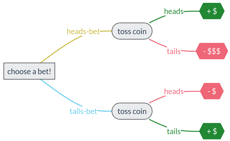
Imagine two persons, Henry and Tina, who must choose between a “heads-bet” or a “tails-bet” before a coin is tossed. The bets are these:
“heads-bet”: If the coin lands heads, the person wins a small amount of money. But if it lands tails, they lose a large amount of money.
“tails-bet”: If the coin lands tails, the person wins a small amount of money. If it lands heads, they lose the same small amount of money.
Here’s a graphical representation of the situation:
Which bet would you choose? why?
Now this happens: Henry chooses the heads-bet. Tina chooses the tails-bet. The coin comes down heads. So Henry wins the small amount of money, while Tina loses the same small amount.
What would we say about their decisions?
Henry’s decision was lucky, and yet irrational: he risked losing much more money than he could win. Tina’s decision was unlucky, and yet rational: she wasn’t risking to lose more than she could win. Said otherwise, the heads-bet had higher risk of loss than the tails-bet, and not even an higher chance of gain. We expect that any person making Henry’s decision in similar, future bets will eventually lose more money than any person making Tina’s decision.
The method we’re looking for is therefore one that, in the hypothetical situation above, would lead to the same decision as Tina’s, even if Tina’s decision was unlucky. That’s the decision that we call rational or optimal in such an uncertain situation.
Our discussion and the distinction between “successful” and “optimal” decisions also show that we cannot evaluate the efficacy of a method for decisions under uncertainty, by checking whether or how often that method leads to the desired, “successful” consequence. This point is also easily illustrated with a variation on Henry and Tina’s example:
Suppose the general context and the bets are exactly the same. But now imagine Henry and Tina to be the names of two automated decision methods, say two machine-learning algorithms. Also, let’s say that you first toss the coin in secret and see its outcome, then you offer the possible bets to Henry and Tina, who are completely ignorant about the outcome (note that no cheating is involved).
You toss the coin and see that it lands heads. Then the choice of bets is offered to Henry and Tina. Henry chooses the heads-bet and Tina the tails-bet.
Now consider this: you know the “truth”, you know what the successful decision would be: heads-bet. It turns out that the Henry algorithm made the choice corresponding to the truth. The Tina algorithm didn’t. Would you then evaluate the Henry algorithm to be better than the Tina algorithm?
For exactly the same reasons already discussed, the Tina algorithm is the better one; it made the optimal decision. Yet it didn’t choose the “truth”. You realize that comparing algorithms is not as simple as checking which one yields the truth.
We have then arrived at two conclusions:
- “Success” or “correspondence to truth” is generally not a good criterion to judge a decision under uncertainty or to evaluate an algorithm that makes such decisions. Moreover, in real applications the truth is not known – that’s the whole problem! – so how can we use a criterion based on truth?
- Even if there is no method to determine which decision is successful, there is nevertheless a method to determine which decision is rational or optimal, given the particular gains, losses, and uncertainties involved in the decision problem.
We had a glimpse of this method in our introductory scenarios with electronic components and their variations.
Let us emphasize, however, that we are not giving up on “success”; nor are we trading “success” for “optimality”. We’ll find out that Decision Theory automatically leads to the successful decision in problems where uncertainty is not present or is irrelevant. It’s a win-win. Keep this point firmly in mind:
We shall later witness this fact with our own eyes. We will also take it up in the discussion (chapter 43) of some misleading techniques to evaluate machine-learning algorithms.
2.5 Decision Theory
So far we have mentioned that Decision Theory has the following features:
It tells us what’s optimal and, when possible, what’s successful.
It takes into consideration decisions, consequences, costs and gains.
It is able to deal with uncertainties.
What other kinds of features should we demand from it, in order to be applied to as many kinds of decision problems as possible, and to be relevant for data science? Here are two:
If we find an optimal decision in regards to some problem, it may still happen that this decision leads to new, subsequent decision problems. For example, in the assembly-line scenario the decision
discardcould be carried out by burning, recycling, and so on. And each of these actions could have uncertain results and costs or gains. We thus face a decision after a decision, or a decision within a decision. In general, a decision problem may involve several decision sub-problems, in turn involving decision sub-sub-problems, and so on.In data science, a common engineering goal is to design and build an automated AI-based device capable of making an optimal decision, at least in specific kinds of uncertain situations. Think for instance of an aeronautic engineer designing an autopilot system; or a software company designing an image classifier.
Well, Decision Theory turns out to meet these two demands too, thanks to the following features:
It allows for recursive, sequential, and modular application.
It can be used not only for human decision-makers, but also for AI or automated devices.
Decision Theory has a long history, going back to Leibniz in the 1600s and partly even to Aristotle in the −300s. It appeared in its present form around 1920–1960, from the contributions of Wald, von Neumann and Morgenstern, Savage, and many others. What’s remarkable about it is that it is not only a framework: it is the framework we must use. A logico-mathematical theorem shows that any framework that does not break basic optimality and rationality criteria has to be equivalent to Decision Theory. In other words, an “alternative” framework might use different terminology and apparently different mathematical operations, but it would boil down to the same notions and mathematical operations of Decision Theory. So if you wanted to invent and use another framework, then either (a) your framework would lead to some irrational or illogical consequences; or (b) your framework would lead to results identical to Decision Theory. Many frameworks that you are probably familiar with, such as optimization theory or Boolean logic, are just specific applications or particular cases of Decision Theory.
Thus we list one more important characteristic of Decision Theory:
- It is normative.
Normative contrasts with descriptive. The purpose of Decision Theory is not to describe, for example, how human decision-makers typically make decisions. Human decision-makers typically make irrational, sub-optimal, or biased decisions. That’s exactly what we want to avoid! We want a theory, a norm, that human decision-makers should aspire to. That’s what Decision Theory is.