39 Introduction to machine learning
\(\DeclarePairedDelimiter{\set}{\{}{\}}\) \(\DeclarePairedDelimiter{\abs}{\lvert}{\rvert}\)
So far we have learned about the principles behind drawing inferences and making decisions, and about various properties of data. Using only the four fundamental probability rules that drive the “thinking” of a perfect AI agent, we arrived at a couple of formulae that underlie many different kinds of inference, prediction, and data-generation tasks, in situations where the agent believe the data to be exchangeable (ch. 25). One example is
\[ \begin{aligned} &\mathrm{P}\bigl( \color[RGB]{238,102,119}Y_{N+1} \mathclose{}\mathord{\nonscript\mkern 0mu\textrm{\small=}\nonscript\mkern 0mu}\mathopen{}y_{N+1} \color[RGB]{0,0,0}\pmb{\nonscript\:\vert\nonscript\:\mathopen{}} \color[RGB]{34,136,51}X_{N+1} \mathclose{}\mathord{\nonscript\mkern 0mu\textrm{\small=}\nonscript\mkern 0mu}\mathopen{}x_{N+1}\, \mathbin{\mkern-0.5mu,\mkern-0.5mu}\, Y_N \mathclose{}\mathord{\nonscript\mkern 0mu\textrm{\small=}\nonscript\mkern 0mu}\mathopen{}y_N \mathbin{\mkern-0.5mu,\mkern-0.5mu}X_N \mathclose{}\mathord{\nonscript\mkern 0mu\textrm{\small=}\nonscript\mkern 0mu}\mathopen{}x_N \mathbin{\mkern-0.5mu,\mkern-0.5mu} \dotsb \mathbin{\mkern-0.5mu,\mkern-0.5mu} Y_1 \mathclose{}\mathord{\nonscript\mkern 0mu\textrm{\small=}\nonscript\mkern 0mu}\mathopen{}y_1 \mathbin{\mkern-0.5mu,\mkern-0.5mu}X_1 \mathclose{}\mathord{\nonscript\mkern 0mu\textrm{\small=}\nonscript\mkern 0mu}\mathopen{}x_1 \color[RGB]{0,0,0}\mathbin{\mkern-0.5mu,\mkern-0.5mu}\mathsfit{I}\bigr) \\[2ex] &\qquad{}= \frac{ \sum_{\boldsymbol{f}} f({\color[RGB]{238,102,119}Y\mathclose{}\mathord{\nonscript\mkern 0mu\textrm{\small=}\nonscript\mkern 0mu}\mathopen{}y_{N+1} \mathbin{\mkern-0.5mu,\mkern-0.5mu}\color[RGB]{34,136,51}X\mathclose{}\mathord{\nonscript\mkern 0mu\textrm{\small=}\nonscript\mkern 0mu}\mathopen{}x_{N+1}}) \cdot f({\color[RGB]{34,136,51}Y\mathclose{}\mathord{\nonscript\mkern 0mu\textrm{\small=}\nonscript\mkern 0mu}\mathopen{}y_{N} \mathbin{\mkern-0.5mu,\mkern-0.5mu}X\mathclose{}\mathord{\nonscript\mkern 0mu\textrm{\small=}\nonscript\mkern 0mu}\mathopen{}x_{N}}) \cdot \, \dotsb\, \cdot f({\color[RGB]{34,136,51}Y\mathclose{}\mathord{\nonscript\mkern 0mu\textrm{\small=}\nonscript\mkern 0mu}\mathopen{}y_{1} \mathbin{\mkern-0.5mu,\mkern-0.5mu}X\mathclose{}\mathord{\nonscript\mkern 0mu\textrm{\small=}\nonscript\mkern 0mu}\mathopen{}x_{1}}) \cdot \mathrm{P}(F\mathclose{}\mathord{\nonscript\mkern 0mu\textrm{\small=}\nonscript\mkern 0mu}\mathopen{}\boldsymbol{f}\nonscript\:\vert\nonscript\:\mathopen{} \mathsfit{I}) }{ \sum_{\boldsymbol{f}} f({\color[RGB]{34,136,51}X\mathclose{}\mathord{\nonscript\mkern 0mu\textrm{\small=}\nonscript\mkern 0mu}\mathopen{}x_{N+1}}) \cdot f({\color[RGB]{34,136,51}Y\mathclose{}\mathord{\nonscript\mkern 0mu\textrm{\small=}\nonscript\mkern 0mu}\mathopen{}y_{N} \mathbin{\mkern-0.5mu,\mkern-0.5mu}X\mathclose{}\mathord{\nonscript\mkern 0mu\textrm{\small=}\nonscript\mkern 0mu}\mathopen{}x_{N}}) \cdot \, \dotsb\, \cdot f({\color[RGB]{34,136,51}Y\mathclose{}\mathord{\nonscript\mkern 0mu\textrm{\small=}\nonscript\mkern 0mu}\mathopen{}y_{1} \mathbin{\mkern-0.5mu,\mkern-0.5mu}X\mathclose{}\mathord{\nonscript\mkern 0mu\textrm{\small=}\nonscript\mkern 0mu}\mathopen{}x_{1}}) \cdot \mathrm{P}(F\mathclose{}\mathord{\nonscript\mkern 0mu\textrm{\small=}\nonscript\mkern 0mu}\mathopen{}\boldsymbol{f}\nonscript\:\vert\nonscript\:\mathopen{} \mathsfit{I}) } \end{aligned} \tag{39.1}\]
We saw that the agent needs to have a built-in belief about frequencies, \(\mathrm{P}(F\mathclose{}\mathord{\nonscript\mkern 0mu\textrm{\small=}\nonscript\mkern 0mu}\mathopen{}\boldsymbol{f}\nonscript\:\vert\nonscript\:\mathopen{} \mathsfit{I})\). Once it’s given some learning data, it can in principle draw all sorts of inferences and make all sorts of decisions. Concrete applications were given in chapters 33, 34, 37.
We shall now discuss about some present-day approximate procedures to draw inferences about data. They are approximate because they draw inferences or make decisions by doing approximate probability calculations and approximate maximizations of expected utilities, rather than exact ones. This approximating character makes these procedures very fast, but also sub-optimal. In any given problem it is therefore important to decide whether our priority is speed or optimality.
Machine learning methods can be wildly different both in terms of operation and complexity. But they all behave as functions that take in a data point \(x\), a set of values \(\mathbf{w}\) which we call parameters, and returns the prediction \(\hat{y}\):
\[ \hat{y} = f(x, \mathbf{w}). \tag{39.2}\]
The prediction \(\hat{y}\) can be any quantity discussed in section 12.2 – most commonly we want to classify the data (and we say we are doing classification), or we want to estimate some value (in which case we call it regression).
It has been pointed out already – and we will see it also in the coming chapters – that often there is actually not a functional relationship between the inputs \(\mathbf{x}\), and the property we want to predict. This leaves us with two possibilities for a solution:
- If there is an approximate functional relationship, we can try to find an analytical function to model that. More specifically, we can look for a deterministic function, which for a given input \(x\) will repeatedly give an output \(y\). Common machine learning methods will work well here.
- If there is no functional relationship, it does not make sense to make a model that tries to enforce one. Instead of having a model that outputs a deterministic value, we need instead, is one that outputs a probability distribution.
Because of the second point above, when we describe equation 39.2, we will use the word “function” in the wide sense where we allow it to be non-deterministic. An example is ChatGPT, which will answer you differently if you ask it the same exact question twice. If you prefer more mathematical rigour, we could call \(f\) a process instead, which is a more loose term.
Let us break down equation 39.2. As engineers, when faced with the task of using data to model the behaviour of some system, our job is twofold. First, we need to select a suitable method to serve as the function \(f\), and second, we need to find the optimal values for the parameters \(\mathbf{w}\). In ADA501 we will see how to choose an analytical \(f\) that corresponds to certain physical systems, while in our course, we will look at methods where \(f\) can be practically anything.
Finding the parameters \(\mathbf{w}\) is what takes us from a general method, to the specific solution to a problem. As we will see, the way of finding them differs between the various machine learning methods, but the principle is always the same: We need to choose a loss function, and then iteratively adjust \(\mathbf{w}\) so that the loss, when computed on known data, becomes as small as possible. The loss function should represent the difference between what the model outputs, and the correct answer – the better the model, the smaller the difference. The choice of this loss function depends on what kind of problem we wish to solve, and we will look at the common ones shortly. But at this point we can already define the three main types of machine learning:
- If we know the “correct answers” (the labels) for all entries in our data set, this is what the model should aim to learn, and we call it supervised learning.
- If we do not have the data labels, we can still write a loss function corresponding to what we want the model to do with the data. Most commonly, we want to find groups, or clusters, of similar-looking data points. If we provide a way of computing scores for good clusters, the model is left to find cluster labels by it self, and we call it unsupervised learning.
- If the decision of a model on one data point affects the value of future data points, like for a self-driving car that may turn left and crash, or turn right and follow the road, we need a loss function that penalises certain actions and rewards others. This is called reinforcement learning.
Having decided on a method to represent \(f\) and found a set of parameters \(\mathbf{w}\), we say that these combined now constitute our model. The model should have internalised the important correlations in the data and thereby allows us to make predictions, i.e. do modelling. If we do decision-making based on the output of the model as well, we typically call in an agent, since there is now some level of autonomy involved. In this chapter, however, we will stick to modelling problems in a supervised fashion.
39.1 Hyperparameters and model complexity
You may have heard the quote by statistician George Box:
All models are wrong, but some are useful.
Although coming off as a somewhat negative view on things, the quote still captures an important point about statistical modelling – our goal is not to make a complete, 100% accurate description of reality, but rather a simplified description that is meaningful in the context of our task at hand. The “correct” level of simplicity, in other words the optimal number of parameters \(\mathbf{w}\), can be hard to find. Often it will be influenced by practical considerations such as time and computing power, but it is always governed by the amount of data we have available. We will look at the theory of model selection later, but let us first consider a visual example, from which we can define some important concepts.
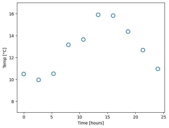
Imagine that you don’t have a thermometer that shows the outside temperature. Never knowing whether you should wear a jacket or not when leaving the house, you get a great idea: If you can construct a mathematical model for the outside temperature as a function of the time of day, then a look at the clock would be enough to decide for or against bringing a jacket. You manage to borrow a thermometer for a day, and make ten measurements at different times, which will form the basis for the model:
The next step is to choose a function \(f\). For one-dimensional data like this, we could for instance select among the group of polynomials, of the form
\[ f (x, \mathbf{w}) = w_0 + w_1 x + w_2 x^2 + \dots + w_M x^M = \sum_{j=0}^{M} w_j x^j \,, \]
where \(M\) is the order of the polynomial. Recall that a zero’th order polymonial is just a constant value, so such a model would be represented with one single parameter. A first-order polynomial is a linear function (two parameters), and the higher in order (and number of parameters) we go, the more “curves” the function can have. This already presents us with a problem. Which order polynomial (i.e. which value of \(M\)) should we choose? Let us try different ones, and for each case, fit the parameters, meaning we find the parameter values that yield the smallest difference from the measured data points:
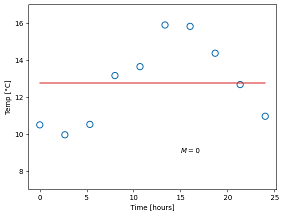
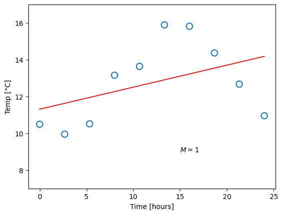
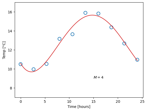
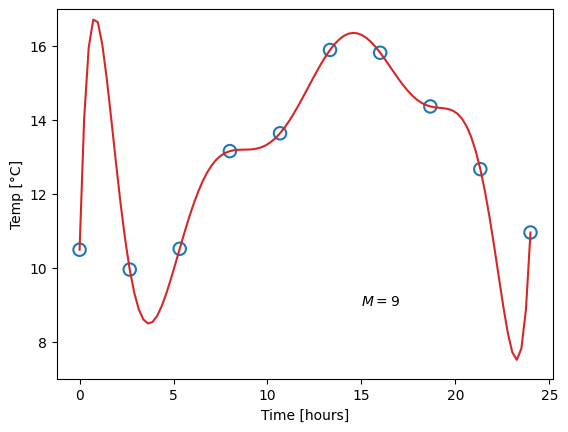
Obviously, the constant function does a poor job of describing our data, and likewise for the linear function. A fourth-order polynomial, on the other hand, looks very reasonable. Now consider the ninth-order polynomial: it matches the measurements perfectly, but surely, this does not match our expectation for what the temperature should look like.
We say that the first and second model underfit the data. This can happen for two reasons: Either the model has too little complexity to be able to describe the data (which is the case in this example), or, potentially, the optimal parameter values have not been found. The opposite case is overfitting, as shown for the last model, where the complexity is too high and the model adapts to artifacts in the data.
This concept is also called the bias-variance tradeoff. We will not go into too much detail on this yet, but qualitatively, we can say that bias (used in this setting) is the difference between the predicted value and the true value, when averaging over different data sets. Variance (again when used in this setting) indicates how big the change in parameters, and hence in model predictions, we get from fitting to different data sets. Let us say you measure the temperature on ten different days, and for each day, you fit a model, like before. These may be the results:
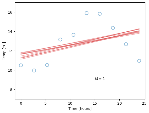
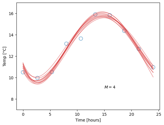
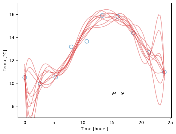
The blue dots are our “original” data points, plotted for reference, while the red lines corresponds to models fitted for each day’s measurements. Due to fluctuations in the measurements, they are different, but note how the difference is related to the model complexity. Our linear models (\(M=1\)) are all quite similar, but neither capture the pattern in the data very well, so they all have high bias. The overly complex models (\(M=9\)) have zero bias on their repective dataset, but high variance. The optimal choice is likely somewhere in-between (hence the tradeoff), as for the \(M=4\) models, which perform well without being overly sensitive to fluctuations in data. Since the value of \(M\) is chosen by us, we call it a hyperparameter, to separate it from the regular parameters which are optimised by minimising the loss function.
Exercise 39.1
Our simple temperature model relies on a series of assumptions, some which might be good, and some which might be (very) bad. State the ones you can think of, and evaluate if they are sensible. Hints: are polynomials a good choice for \(f\)? Is the data representative?
For the different models in figure 39.2 we started by choosing polymonial degree \(M\), and then computed the parameters that minimized the difference between the data points and the model. Then we had a look at the results, compared them to our expectations, and decided that \(M=0\) and \(M=9\) were both unlikely. Can you think of a way to incorporate our initial expectations into the computation?
39.2 Model selection (in practice)
As alluded to in the exercises above, there are ways of including both the data and our prior expectations when building a model, but it is, in fact, not very common to do so. In this section we will have a look at the typical machine learning approach, which relies on splitting the data in different sets. Starting from all our available data on a given problem that we wish to model, we divide it into
- the training set, which is the data we will use to determine the model parameters \(\mathbf{w}\),
- the validation set, which is used to evaluate the model complexity (i.e. finding the optimal bias-variance tradeoff), and
- the test set, which is used to evaluate the final performance of the model.
The benefit of this approach is that it is very simple to do. The downside, on the other hand, is that each set is necessarily smaller than the total, which subjects us to increased statistical uncertainty. The final parameters will be slightly less optimal than they could have been, and the measurement of the performance will be slightly less accurate. Still, it is common practice, and for the “standard” machine learning methods there is no direct way of simultaneously optimising for the model complexity.
39.3 Overfitting and underfitting: why? where from?
Up to now we have never met the problems of overfitting and underfitting. The OPM agent that we applied in chapters 33, 34, 37 did not suffer from this kind of problems. In fact, in § 33.5 we saw that the agent trained with just 10 datapoints did not try to fit them perfectly, but kept more conservative beliefs. The agent also warned us that further learning data might substantially change its beliefs. When a substantial amount of learning data was given to the agent, it aligned its beliefs with the observed frequencies, which was a reasonable thing to do. No issues about over- or under-fitting appeared at any stage; we did not even think about them.
Why do the machine-learning models above suffer from these issues instead? Where do these issues originate from?
The origins are various and may differ from one machine-learning algorithm to another. In the cases above there are two main culprits:
- a particular approximation underlying the algorithms;
- unreasonable prior beliefs built into the algorithms.
Let’s explain each in broad terms.
The “max instead of sum” approximation
A machine-learning algorithm like one of the above is an agent that tries to predict the \(\mathit{temp}\)erature from the \(\mathit{time}\) by assuming that there’s a function from time to temperature; this could be a reasonable assumption. In loose probability notation we could write it like this:
\[ \mathrm{P}(\mathit{temp} \nonscript\:\vert\nonscript\:\mathopen{} \mathit{time} \mathbin{\mkern-0.5mu,\mkern-0.5mu}F \mathbin{\mkern-0.5mu,\mkern-0.5mu}\mathsfit{I}) \]
where \(F\) represents the assumed function.
But the agent doesn’t know what the true function \(F\) is: it could be the function \(F_{1}\) (say, a line like \(\mathit{temp} = A \cdot \mathit{time} + B\)), or \(F_{2}\) (say, a sine like \(\mathit{temp} = A \cdot \sin(B \cdot \mathit{time}) + C\)), or an infinity of other possibilities. Each function is a hypothesis that the agent is entertaining. Therefore what the agent is trying to calculate is actually something like this:
\[ \mathrm{P}\bigl(\mathit{temp} \nonscript\:\vert\nonscript\:\mathopen{} \mathit{time} \mathbin{\mkern-0.5mu,\mkern-0.5mu} (F_{1} \lor F_{2} \lor \dotsb) \mathbin{\mkern-0.5mu,\mkern-0.5mu}\mathsfit{I}\bigr) \]
A perfect agent, reasoning according to the four fundamental rules, would in this case apply the law of extension of the conversation (§ 9.5), with a sum over the possible function hypotheses:1
1 For simplicity we assume that \(\mathit{time}\) alone is irrelevant for the belief about \(F\).
\[ \mathrm{P}\bigl(\mathit{temp} \nonscript\:\vert\nonscript\:\mathopen{} \mathit{time} \mathbin{\mkern-0.5mu,\mkern-0.5mu} (F_{1} \lor F_{2} \lor \dotsb) \mathbin{\mkern-0.5mu,\mkern-0.5mu}\mathsfit{I}\bigr) = \sum_i \mathrm{P}(\mathit{temp} \nonscript\:\vert\nonscript\:\mathopen{} \mathit{time} \mathbin{\mkern-0.5mu,\mkern-0.5mu}F_{i} \mathbin{\mkern-0.5mu,\mkern-0.5mu}\mathsfit{I}\bigr) \cdot \mathrm{P}(F_{i} \nonscript\:\vert\nonscript\:\mathopen{} \mathsfit{I}\bigr) \]
This law in fact underlies formula 39.1, which we used for our OPM agent. In that formula the sum over hypotheses appears as “\(\sum_{\boldsymbol{f}}\)”, with the difference that the hypotheses in that case were frequencies.
The sum over hypotheses can be computationally expensive, and the machine-learning agents above approximate it with something simpler: they search for, and keep only the largest term in the sum, rather than performing the sum:
\[ \sum_i \mathrm{P}(\mathit{temp} \nonscript\:\vert\nonscript\:\mathopen{} \mathit{time} \mathbin{\mkern-0.5mu,\mkern-0.5mu}F_{i} \mathbin{\mkern-0.5mu,\mkern-0.5mu}\mathsfit{I}\bigr) \cdot \mathrm{P}(F_{i} \nonscript\:\vert\nonscript\:\mathopen{} \mathsfit{I}\bigr) \mathrel{\color[RGB]{238,102,119}\pmb{\approx}} \max_i\Bigl\{ \mathrm{P}(\mathit{temp} \nonscript\:\vert\nonscript\:\mathopen{} \mathit{time} \mathbin{\mkern-0.5mu,\mkern-0.5mu}F_{i} \mathbin{\mkern-0.5mu,\mkern-0.5mu}\mathsfit{I}\bigr) \cdot \mathrm{P}(F_{i} \nonscript\:\vert\nonscript\:\mathopen{} \mathsfit{I}\bigr) \Bigr\} \]
You will see the appearance of this maximization, disguised as a minimization (of minus the logarithms of the sum terms), in the next machine-learning chapters.
In a manner of speaking we can say that a perfect agent makes a prediction by appropriately balancing all unknown alternatives, whereas the approximate machine-learning agent only considers the most “attention-calling” alternative. This is actually a form of cognitive bias, related to the so-called anchoring and availability biases.
To make things worse, the factor \(\mathrm{P}(F_{i} \nonscript\:\vert\nonscript\:\mathopen{} \mathsfit{I})\), which should express prior information about the possible hypothesis \(F_{i}\), is often poorly chosen or not chosen at all, and approximately the same for all hypotheses. So the maximum is effectively determined only by the factor \(\mathrm{P}(\mathit{temp} \nonscript\:\vert\nonscript\:\mathopen{} \mathit{time} \mathbin{\mkern-0.5mu,\mkern-0.5mu}F_{i} \mathbin{\mkern-0.5mu,\mkern-0.5mu}\mathsfit{I}\bigr)\), which expresses how well hypothesis \(F_{i}\) fits the existing data. This leads to overfitting.
One way to mitigate this problem is by not using the maximum among the sum terms, but a somewhat smaller term than the maximum. But how much smaller should it be? In order to evaluate that, a validation dataset is usually introduced, to get an idea at how badly the approximate agent predicts new data while trying to overfit the old data. This is also an approximate make-do solution, however, which still does not lead to the optimal result.
Another way to mitigate the problem is by providing a non-constant prior-belief factor \(\mathrm{P}(F_{i} \nonscript\:\vert\nonscript\:\mathopen{} \mathsfit{I})\); this is what regularization procedures do. However, these procedures do not choose a value based on prior information; the choice is based on blind, trial-and-error attempts to reduce the influence of the data-fit term \(\mathrm{P}(\mathit{temp} \nonscript\:\vert\nonscript\:\mathopen{} \mathit{time} \mathbin{\mkern-0.5mu,\mkern-0.5mu}F_{i} \mathbin{\mkern-0.5mu,\mkern-0.5mu}\mathsfit{I}\bigr)\). The result is again not optimal.
These are the reasons why a perfect agent, such as the OPM of the previous chapters, does not need a validation dataset or regularization procedures: it does not approximate the required sum over hypotheses by a maximization, and it uses meaningful prior information.
Unreasonably restrictive built-in beliefs
For a reasonable prediction it is of course important that the actual function \(F\) is actually among the hypotheses built into the agent. No amount of learning data will increase the agent’s belief in a hypothesis that it isn’t even considering:
\[ \mathrm{P}\bigl(\mathit{temp} \nonscript\:\vert\nonscript\:\mathopen{} \mathit{time} \mathbin{\mkern-0.5mu,\mkern-0.5mu} (\underbracket{\color[RGB]{0,0,0}F_{1} \lor F_{2} \lor \dotsb}_{\color[RGB]{119,119,119}\text{true $F$ missing!}}) \mathbin{\mkern-0.5mu,\mkern-0.5mu}\mathsfit{I}\bigr) \]
No matter how many learning data are used, such an agent will keep on making poor predictions. This leads to underfitting.
Restricting an agent’s set of beliefs in this way is often used to mitigate the “max instead of sum” approximation. We can put this idea in a funny way: since the approximating agent is not balancing all alternatives but only choosing the most attention-calling one, let’s at least give it unreasonable alternatives to maximize from.
39.4 Machine learning taxonomy
Machine learning has been around for many decades, and the list of methods that fit under our simple definition of looking like equation 39.2 and learning their parameters from data, is very long. For a (non-exhaustive) systematic list, have a look at the methods that are implemented in scikit-learn, a Python library dedicated to data analysis.
In this course we will not try to go through all of them, but rather focus on the fundamentals of what they all have in common. With this fundamental understanding, learning about new methods is like learning a new programming language – each has their specific syntax and specific uses, but the underlying mechanism is the same. We will look at two important methods, that are inherently very different, but still accomplish the same end result. The first is decision trees (and the extension into random forests), while the second is neural networks.